NGC1052-DF2: supplementary information
(update October 22, 2018)
NGC1052-DF2 is a galaxy in the NGC1052 group, discovered by Karachentsev et al. (2000). We identified it in a search for low surface brightness objects with the Dragonfly Telephoto Array, and obtained follow-up HST, Keck, and Gemini observations. We initially published two papers on the galaxy; one in Nature on its low dark matter content and one in ApJ Letters on its unusual globular cluster population. The Nature paper, in particular, generated intense interest and also skepticism, as well as a psychological analysis of the authors. More constructively, a paper in ApJ Letters (Martin et al. 2018) explores the confidence limits on the dispersion measurement and a paper submitted to MNRAS (Trujillo et al. 2018) asks whether the galaxy could be at a smaller distance than our measurement.
We have done further work on NGC1052-DF2. First, we unearthed additional LRIS data on one of the globular clusters in NGC1052-DF2, and published a new velocity of this cluster in a AAS Research Note. Responding to a request by the Editors of ApJ Letters and RNAAS we also briefly discuss the Martin et al. (2018) analysis in this Note. In response to the questions about the distance to the galaxy we published an ApJ Letter, demonstrating that Trujillo et al. almost certainly confused blends for isolated stars in their analysis. (At the time of writing the Trujillo paper is still under review, so technically theirs is a response to ours.) We also provide a new distance measurement that is independent of absolute calibrations and nearly identical to our previous result. Yotam Cohen published an analysis of all 23 objects in our Cycle 23 HST program, including NGC1052-DF2. Asher Wasserman wrote an ApJ Letter on the mass constraints, using Jeans modeling of generalized NFW profiles in a Bayesian framework.
Initially much of the information that is in the above-mentioned papers was only provided on this web page. The papers obviously supersede the analysis here; in the weeks following the publication of the papers we worked quickly to provide responses to sometimes-fierce criticism, and sometimes adjusted things when we actually wrote the papers. We planned to remove the information below, but in the end it seems appropriate to keep it here - also because there are some nice graphics that people might find useful. The following is written by the first author (and any criticism should be directed at him), but I am happy to acknowledge Shany Danieli and Yotam Cohen who helped with key aspects. Also, thanks to Nicolas Martin, Michelle Collins, Sam Vaughan, Stacy McGaugh, Nacho Trujillo, and others, for their interest in this result and their critical assessment of it; this is how we make progress!
The following information is superseded by published papers and no longer up to date!
The distance to NGC1052-DF2
We begin by examining the distance to the galaxy, as this discussion has taken on a new urgency in light of the recent arXiv posting by Trujillo et al. For impatient readers: We believe the distance of Trujillo et al. is ruled out by the non-detection of red giant branch stars in NGC1052-DF2, as demonstrated in this image. We appreciate that it may appear somewhat facetious to reply to the comprehensive and carefully written Trujillo et al. paper with a single image, but this is the essence of the debate: for a distance of 13 Mpc the data should comfortably reach below the tip of the giant branch, whereas for 19 Mpc the data should not - there is just no way around this. In the following, and in the paper that we submitted to ApJ Letters, we provide the details.
The distance is something we worried about a lot, from the beginning, for many of the reasons outlined in Nacho's paper: if the galaxy is a factor of two or three closer to us than the adopted distance of 20 Mpc nearly all the unusual properties vanish: its inferred stellar mass goes down, leading to a more comfortable ratio between dynamical mass and stellar mass; its size goes down, meaning it is not a UDG but a dwarf spheroidal, and the luminosities and sizes of its globular clusters are perfectly ordinary. The only odd aspects that are truly independent of distance are the ratio of the luminosity in globular clusters to the total luminosity (which is very high at 3%) and (perhaps) the flattening of the globular clusters (most globular clusters are round, but the ones in DF2 have a mean ellipticity of about 0.2).
There is circumstantial evidence for a distance of about 20 Mpc: the proximity (in projection) to the galaxy NGC1052, and, particularly, the radial velocity of 1800 km/s. This velocity corresponds to a Hubble flow distance of about 25 Mpc, and if the galaxy were at 13 Mpc it would have a peculiar velocity of 900 km/s even though it would live in a very sparsely populated region of space and not in a group. As shown in Figs. 17, 18, and 19 in Trujillo et al., NGC1052-DF2 would have the highest positive peculiar velocity of any known galaxy in a 500 square degree region centered on NGC1052. (Note that the red histogram, not the black histogram, in Fig. 19 is the one for this region of the sky.) Trujillo et al. suggest it might be at the same distance as NGC 1042, but given the large velocity difference with this galaxy (~640 km/s) and its large separation on the sky it would certainly not be bound to it. However, we agree that this argument is not sufficiently persuasive when set against the odd properties of NGC1052-DF2 for a distance of 20 Mpc: it's difficult to make the argument that an extreme peculiar velocity is less likely than a very low dark matter content or a set of extra-luminous globular clusters.
Fortunately independent information is available, from the appearance of the galaxy in the HST images. The galaxy is marginally resolved: some individual stars are detected against a background of surface brightness fluctuations. We used these surface brightness fluctuations (SBF) to determine the distance, arriving at D=19.0+-1.7 Mpc. Trujillo et al. note that the SBF method is difficult to calibrate at blue colors. They use our measurement of the apparent fluctuation magnitude and different ways to calibrate the absolute fluctuation magnitude, finding distances ranging from 14.7 Mpc to "well beyond 25 Mpc". They settle on the nearer distance largely based on SBF distances to a large sample of (luminous) Virgo galaxies from Cantiello, Blakeslee, et al. (2018). We note here that Michele Cantiello and John Blakeslee independently analyzed the NGC1052-DF2 data. They started with the flc images and used their own methods that they developed over the past decade (and used in Cantiello et al. 2018). They find a preliminary distance of D=22+-3 Mpc for NGC1052-DF2 (J. Blakeslee, private communication), slightly larger than (but fully consistent with) our measurement.
Trujillo et al. further argue that the larger SBF distances must be incorrect because the galaxy is resolved into stars, and they determine a distance using the tip of the red giant branch (TRGB) of 13.1 Mpc. However, we believe that they are confusing blends for isolated stars. Blends produce a "phantom" TRGB above the true TRGB. This is a well known effect - see, e.g., Bailin et al. (2011). The only isolated stars that are detected in NGC1052-DF2 are on the AGB, not the RGB. We demonstrate all this in two distinct ways: empirically, from a comparison with other galaxies in our Cycle 24 program, and then by comparing the galaxy to fully-populated model galaxies. (This work was all done prior to the Trujillo et al. paper: we worked on the distance question from the beginning, and we also iterated on this question with another group who suspected that they had detected the TRGB in the HST data). Please see the submitted ApJ Letter for a comprehensive discussion and additional figures.
Comparison of NGC1052-DF2 to other galaxies:
Besides NGC1052-DF2 we observed 23 other low surface brightness "blobs" in our Cycle 24 program. All were identified with Dragonfly; seven are new discoveries. We have submitted a paper describing distance measurements and basic properties for the full sample (Cohen et al. 2018). Below is a comparison between the appearance of the galaxy M96-DF11 (or Leo-DF11 - it is in the Leo/M96 group) in a single orbit to NGC1052-DF2 in two orbits. M96-DF11 has a very similar surface brightness, color, apparent size, and morphology as NGC1052-DF2, but its appearance in the HST data is very different:
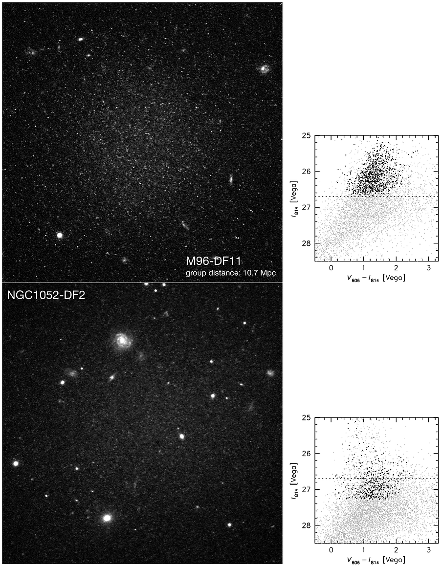
Figure 1. Images of two galaxies from our sample of 23 "blobs" that we imaged in Cycle 24 with HST. M96-DF11 is the closest analog to NGC1052-DF2 in terms of its apparent properties (color, surface brightness and apparent size). M96-DF11 resolves into a sea of stars, as HST reaches the well-populated RGB even in a single orbit for a distance of 10.7 Mpc. Despite its similar total apparent magnitude the number of stars detected above the dotted line is an order of magnitude smaller than in M96-DF11. From van Dokkum et al, 2018, submitted to ApJ Letters.
M96-DF11 is far more resolved than NGC1052-DF2, and this is very clear in the CMDs (shown at right). Grey points in the CMDs are "raw" detections before quality cuts, and black points are the surviving stars after quality cuts. The CMD for NGC1052-DF2 in Trujillo et al. looks far more populated than the one shown above, but similar to the CMD prior to applying quality cuts (grey points). We speculate that their detection algorithm does not apply rigorous cuts to limit the effects of blends. We use DOLPHOT and the standard quality cuts used in this field (see GHOSTS, ANGST, etc papers) to prevent this, but these key steps are not described in Trujillo et al. The importance of this issue is demonstrated below. If no cuts are applied the photometric analysis will mistake all the SBF peaks as stars, and we arrive at a very similar CMD as in Trujillo et al., with an apparent sharp feature at I=26.5. With the standard quality cuts the surface brightness fluctuations are removed from the analysis and only the actual stars remain (these are mostly AGB stars, not stars below the tip of the RGB).
Even after removing blends there is an increase in the number of detections below I~26.5, due to a mix of scattering due to photometric errors, residual blends that are too close to resolve, and AGB stars. We can demonstrate this empirically by shifting the CMDs of galaxies at smaller distances to 19 Mpc:
Figure 2. The CMD of NGC1052-DF2 is far more populated in Trujillo et al. than in our analysis. We can only reproduce the Trujillo CMD if we do not apply quality cuts in our analysis. In the middle panels we turn off all quality cuts, and in the right panel we apply the standard cuts that are used in GHOSTS, ANGST, etc. Without quality cuts we arrive at a very similar CMD as Trujillo et all, with an apparently well defined feature at ~26.5 that they interpret as the TRGB. The bottom panels show the origin of the difference: the quality cuts are crucial to weed out blends (effectively the peaks of surface brightness fluctuations) from the analysis. The structure in between the detections does not consist of individual stars but of clumps of 2-3 stars that are blended together.

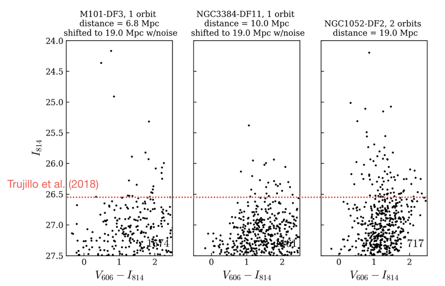
For good measure we also show M101-DF3 in the figure above, a galaxy with a very secure TRGB distance (Danieli et al. 2017). After placing them at 19 Mpc both M101-DF3 and M96-DF11 show a clear "feature" at the apparent TRGB location derived by Trujillo et al: the horizontal line. To emphasize: this is not the TRGB, as M101-DF3 and M96-DF11 were artificially shifted to 19 Mpc for this comparison.
As a final figure in this empirical section we show a comparison of TRGB and SBF distances of all galaxies in our sample - this is from the Cohen et al. paper. This figure shows that the SBF distances that we derive are very nicely consistent with the TRGB distances, in the regime where we can measure both. This addresses the question that Nacho raises about our calibration of the SBF magnitudes. We address this issue also in the ApJ Letter, by deriving a new distance that only uses relative calibrations, starting from the maser galaxy NGC4258.
Figure 3. CMDs of two galaxies in our sample with secure TRGB distances (M101-DF3 at 6.8 Mpc and M96-DF11 at 10.7 Mpc), after shifting the CMDs to 19.0 Mpc and adding the NGC1052-DF2 photometric errors. These are compared to the actual CMD of NGC1052-DF2 on the right. The feature that Trujillo et al. (2018) identify in the CMD of NGC1052-DF2 is indicated with the red dashed line. The same feature is seen in the shifted CMDs, demonstrating that it is not the TRGB but a mix of AGB stars, the effects of photometric errors upscattering stars just below the TRGB, and residual blends. (This is after applying quality cuts that weed out most of the blends.)

Figure 4. Distances of galaxies in our Cycle 24 program, measured from the TRGB and SBF. Grey bands are the distances of the targeted groups. Our TRGB and SBF distances are consistent with each other in the regime where both can be measured, allaying potential concerns about our calibration of the fluctuation magnitudes.
A key point here is that the relative distance between NGC1052-DF2 and the Leo/M96 group galaxies is well-determined, as the calibration errors cancel (these are galaxies with very similar ages, metallicities, and surface brightness): the ratio is about a factor of 1.9. As the M96 group galaxies have secure distances of ~10.7 Mpc from the TRGB (and the Cosmicflows-3 database), we arrive at a distance of approximately 19 Mpc that is independent of the absolute calibration of the surface brightness fluctuation magnitude.
Comparison of NGC1052-DF2 to fully populated model galaxies:
Shany Danieli created a tool ("ArtPop") that can generate artificial galaxy images, using fully populated CMDs from the latest FSPS models. We made "realizations" of NGC1052-DF2 for different distances, assuming old ages and low metallicities, always matching the total apparent magnitude, size, axis ratio, and Sersic of NGC1052-DF2. These models demonstrate directly what happens when the galaxy is shifted to larger distances, and by placing them in an empty region of the actual NGC1052-DF2 images we ensure that we use the correct noise and contamination. The results for distances of 12 and 20 Mpc are shown below. (We used 12 Mpc as this was the distance derived by another group from the same feature in the CMD as Trujillo et al. identify as the TRGB - we will update the figure for 13.1 Mpc)

Figure 5. Models of NGC1052-DF2 made with the ArtPop code (Danieli et al. 2018). These models reproduce the morphology, surface brightness, apparent size, and integrated color of NGC1052-DF2, and use fully populated isochrones from the latest FSPS models to simulate the stellar population. We convolved the models with the HST PSF and placed thems in an empty area of the actual NGC1052-DF2 image. For a distance of 12 Mpc (and 13 Mpc) the galaxy resolves into stars, as HST reaches the giant branch. For D=19 Mpc the model stars blend together into surface brightness fluctuations, as observed.
It is clear, particularly from the bottom row, that the 19 Mpc model is a far better match to the data than the 12 Mpc model: in the 12 Mpc model, the galaxy resolves into a sea of individual giant stars below the TRGB, whereas those same stars blend together into surface brightness fluctuations at 19 Mpc. The reason for this relatively strong distance-dependent behavior is that surface brightness is conserved in all models (as is required to match the observations). As a result, for an increase in the distance of a factor of 2, not only do the stars get fainter by a factor of 4, there are also 4x more of them. This is why the transition from resolved stars to surface brightness fluctuations is quite rapid: for a factor of 2 increase in distance, each star is replaced by 4 fainter ones.
Finally, we show the outer regions of the models and of NGC1052-DF2. There, the giants are so far apart that the transition to surface brightness fluctuations does not occur: instead, they simply become undetectable:
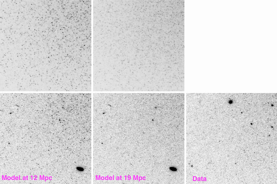
The figure clearly shows that individual stars on the RGB can be detected with HST in two orbits at 12 Mpc but not at 19 Mpc (as is well known). The data look nearly identical to the 19 Mpc model, with many faint 2-3σ smudges that would turn into detections with deeper data. The data look very different from the 12 Mpc model. Boiled down to its essence, our reply to the Trujillo et al. paper is this figure.
The TRGB / SBF measurement should be definitive, in the sense that it has far more weight than the other, conflicting, distance estimators: the unusual globular clusters and the velocity dispersion (or Fundamental Plane, in the phrasing of Trujillo et al.) arguing for a small distance, and the closeness in projection to NGC 1052 plus the Hubble flow distance arguing for a large distance.
Figure 6. Same as Fig. 4, but now focusing on a region in the outskirts with a low stellar density. In the 12 Mpc model stars are easily detected in this region, whereas they are 2-3σ smudges in the 19 Mpc model. This is exactly what is observed in this outer region of NGC1052-DF2: hints of many faint objects just below the detection limit, but only a small number of detected bright stars (note that several of the compact objects in the NGC1052-DF2 image are globular clusters). Click here to download a high resolution version of this image.
-- THE INFORMATION BELOW IS BEING UPDATED ---
Is NGC1052-DF2 a "normal" dwarf?
We begin our in-depth analysis by looking at DF2's morphology and globular cluster population. DF2 is an ultra diffuse galaxy, that is, it has an effective radius >1.5 kpc and a central surface brightness μ(g,0)>24 mag/arcsec^2. Notionally UDGs are dwarf galaxies, at least according to a simple stellar mass or luminosity criterion. Furthermore, there is no evidence for a discontinuity between UDGs and galaxies outside of their particular selection box, at least in any parameter that has been studied so far. However, they really are quite different from Local Group galaxies with the same stellar mass. This is illustrated with the image below, where we have placed fully-modeled versions of NGC 147 and NGC 185 (using the ArtPop code) next to DF2, after moving them to a distance of 20 Mpc.
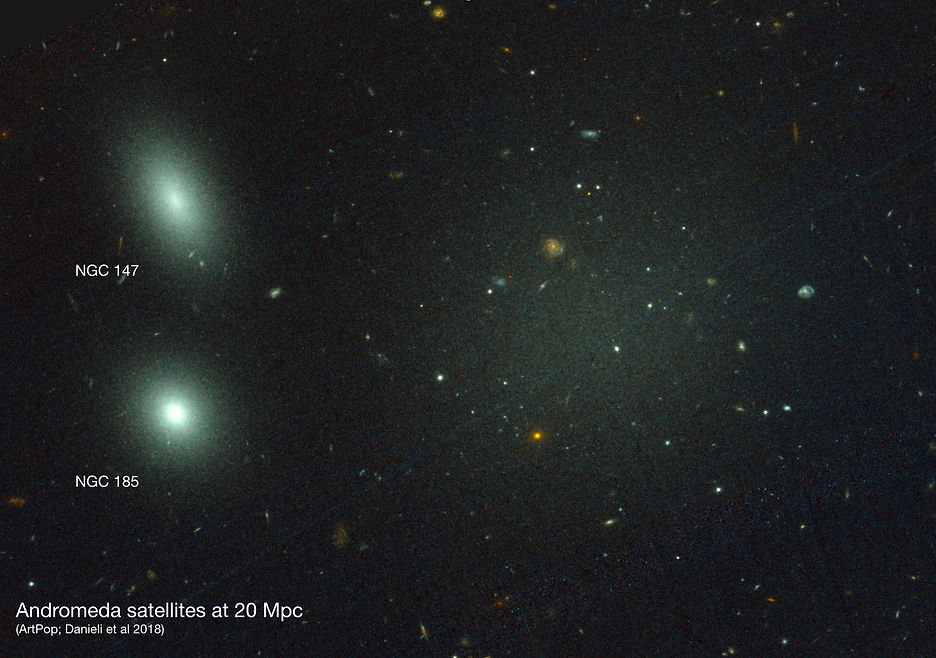
Figure 1. Models of NGC 147 and NGC 185 shifted to 20 Mpc and placed alongside NGC1052-DF2 in our HST imaging. The models consist of all individual stars in the galaxies, and are created with the ArtPop code (Danieli et al. 2018). Inputs were obtained from the Nearby Dwarf Database, plus structural parameters from Geha et al. (2010). The three galaxies in this image have approximately the same stellar mass.
DF2 looks very different from NGC 147 and NGC 185: it is much larger and much more diffuse. With a half-light radius of 2.2 kpc DF2 is actually fairly small for a UDG; Dragonfly 44 in the Coma cluster has a half-light radius of 4.7 kpc. Below is an illustration of the huge size of these things. Here we placed Dragonfly 44 at the distance of Andromeda, i.e., the actual distance of NGC 147 and NGC 185. Its half-light diameter would be 0.8 degrees at that distance, larger than the full moon. NGC1052-DF2 is somewhat smaller, but its globular cluster system would extend over an area that is six times larger than the moon's surface.

Figure 2. Dragonfly 44 is an ultra diffuse galaxy in the Coma cluster, with a half-light diameter of 9.2 kpc. If it were at the distance of M31 its half-light diameter would be 0.8 degrees.
Their large sizes make UDGs very interesting from a dark matter perspective: because they are so diffuse the stellar contribution to the mass is expected to be negligible even in the central regions, and because they are so large they trace the mass profile out to very large radii for galaxies of this stellar mass (nearly 8 kpc, or the radius of the Solar orbit in our Galaxy, for DF2). This is what makes the constraint on the halo mass of DF2 unusually robust: for halo masses around 10^8 Msun the globular clusters trace the mass out to the virial radius of the halo. (For Dragonfly 44 this is not the case: it has a far more massive halo with a virial radius of about 100 kpc, and even though the dispersion of Dragonfly 44 has a relatively small uncertainty its dark matter mass is uncertain by about an order of magnitude. These issues are discussed in the Nature paper, and also in a recent arXiv submission by Laporte et al. Paradoxically, because of the relation between virial radius and halo mass, the lower the halo mass the better constrained it is.)
We note that this has to be taken into account when comparing M/L ratios of UDGs to other galaxies. In particular, Martin et al. (2018) use the M/L ratio within the effective radius as the diagnostic parameter to determine how dark matter-dominated a galaxy is. However, because DF2 is so much larger than NGC 147 and NGC 185 its half-light radius encompasses a far greater fraction of the dark matter halo than the half-light radii of the Andromeda satellites do. Therefore, its M/L ratio within the half-light radius would be about an order of magnitude higher than the M/L ratios of the Andromeda satellites if all three galaxies had the same amount of dark matter. This is what makes our central result, the dark matter-deficiency of DF2, so robust: it is not sensitive to the exact value of (or limits on) the velocity dispersion, as discussed in the Methods section of the paper.
Besides the kinematics the globular cluster system of DF2 is truly remarkable, and we devoted a separate paper to it. These globular clusters imply that DF2 is a unique galaxy completely independently from its kinematics. It has 11 large, luminous, and flattened clusters. The brightest is a near-copy of ω Centauri (the largest and most massive globular cluster in the Milky Way) in terms of its luminosity, stellar population, size, and ellipticity:

Figure 3. GC-73, the brightest globular cluster in NGC1052-DF2. It is a near-copy of ω Centauri, the largest and most luminous globular cluster in the Milky Way, in terms of its stellar population, mass, and structure. Note the extreme contrast in surface density between GC-73 and the background light of DF2.
It is difficult to visualize the dramatic nature of the globular clusters in DF2, but we make an attempt in the figure below. Here we show the globular clusters in DF2 (actually, their best fitting King models) projected onto the familiar galaxy NGC 147. The luminosities and sizes of the galaxy and the globular clusters are modeled in a self-consistent way, so they can be compared directly. It is immediately clear that we know of no other galaxy with such an extreme population of compact star clusters.

Figure 4. Modeled appearance of NGC 147, if it had the same 11 luminous globular clusters as NGC1052-DF2.
It seems likely that the three stand-out properties of DF2 (the large size, the globular cluster population, and the lack of dark matter) are causally related; and this is discussed in our ApJ Letter. There is also a heuristic argument that can be made here, and it goes as follows: the fact that this galaxy is unique in one property (the globular clusters) makes it more likely that it is also unique in some other property (the lack of dark matter). Needless to say, this is a slippery slope - something that is extremely rare does not necessarily make something else that is extremely rare more likely. However, the argument can be used in reverse: if a galaxy without dark matter exists, it seems likely that it would also be unusual in some other respect. As Stacy McGaugh often points out, if 1000 similar-looking spiral galaxies have a particular dynamic signature, we should be skeptical that the 1001th similar-looking galaxy behaves differently. Quite simply, a galaxy like DF2 has not been studied kinematically before, and we should be open to surprises.
The distance of NGC1052-DF2
The distance of the galaxy is something we worried about a lot, from the beginning. If the galaxy is a factor of two or three closer to us than the adopted distance of 20 Mpc nearly all the unusual properties vanish: its inferred stellar mass goes down, leading to a more comfortable ratio between dynamical mass and stellar mass; its size goes down, meaning it is not a UDG but a dwarf spheroidal, and the luminosities and sizes of its globular clusters are perfectly ordinary. The only odd aspects that are truly independent of distance are the ratio of the luminosity in globular clusters to the total luminosity (which is high at 3%) and the flattening of the globular clusters (most globular clusters are round, but the ones in DF2 have a mean ellipticity of about 0.2).
As discussed in quite some detail in the Nature paper there is not only strong circumstantial evidence for a distance of about 20 Mpc (the radial velocity of 1800 km/s; the proximity, in projection, to the galaxy NGC1052; and the lack of any other known galaxies at closer distances in this general area of the sky), but decisive evidence from the appearance of the galaxy in the HST data. No individual RGB stars are detected in the galaxy (we do detect AGB stars), giving a lower limit to its distance. However, the galaxy light is not entirely smooth but exhibits spatial fluctuations, caused by stochastic variation in the number of giant stars in each pixel. This surface brightness fluctuation signal gives a distance of D=19.0 Mpc, with an uncertainty of about 1.7 Mpc. Given that the radial velocity of DF2 and the SBF signal of NGC1052 itself indicate slightly higher distances, we adopt 20 Mpc in the paper.
This is all explained in some detail in the Methods section - and in even more detail in an upcoming paper by Yotam Cohen on the full sample of 23 objects - but the figure below makes it (hopefully) immediately clear that this is not a subtle issue. Below we compare the appearance of DF2 to that of M101-DF1, a dwarf galaxy that Allison Merritt discovered with Dragonfly in 2014. We observed it with HST later, in the same way as NGC1052-DF2, and Shany Danieli determined the distance with the TRGB method. It is at 7 Mpc, and a satellite of its giant neighbor M101. The galaxy has about the same central surface brightness as DF2, but it looks completely different in the HST images: it is clearly resolved into stars, whereas DF2 is not. There is just no question that DF2 is at a much greater distance.

Figure 5. Appearance of DF2 in the HST data compared to that of the dwarf galaxy M101-DF1 at 7 Mpc. Each panel is 30'' x 30''. NGC1052-DF2 is not resolved into stars, which means it is much farther away than M101-DF1. It does have a "mottled" appearance, due to the pixel-to-pixel variation in the number of giant stars. The amplitude of this variation provides the distance to NGC1052-DF2.
Velocity dispersion measurement
The dark matter measurement rests on a determination of the velocity dispersion of the galaxy. The dispersion is measured from the radial velocities of individual globular clusters in the galaxy. These velocities are given in the Nature paper, with errors that were determined from "shuffling" the residuals of the best fits. The figure below shows the unbinned velocities, with each point represented by a Gaussian "smear" that indicates its uncertainty, along with (in yellow) the 68% confidence limits. Click here for an ASCII table, including distances from the center of the galaxy.
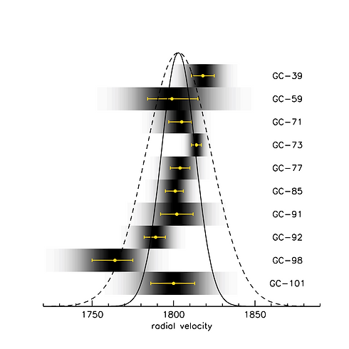
Figure 6. Unbinned velocities, taken straight from the information in Fig. 2 of the Nature paper and simply ordered by rank number. The greyscale shows the (asymmetric) uncertainty for each point, that is, by how much they can be expected to deviate from their true location. The yellow error bars show the 68% confidence limits. The true distribution is expected to be narrower than the observed distribution. The solid line shows a Gaussian with σ=10.5 km/s. This is the 90% confidence upper limit we derive for the intrinsic dispersion (that is, before the distribution is broadened by the observational errors). For reference, the broken line shows a Gaussian with σ=20 km/s.
The error bars cause the observed distribution of velocities to be wider than the intrinsic, true distribution. For a Gaussian intrinsic distribution, Gaussian errors, and a large sample, the intrinsic width can be estimated by subtracting the observational errors in quadrature. Things are more complicated for small samples, when errors are different for each object, and particularly for non-Gaussian distributions. Simple tests for Gaussianity (e.g. the Anderson-Darling test, the Kolmogorov-Smirnov test, and the Shapiro-Wilk test), demonstrate that the observed distribution is significantly non-Gaussian. This is illustrated in Fig. 7, which shows the distribution of the 10 clusters in the variable (Δv)^2, which is what most measures of the scale (width) of a distribution "see":
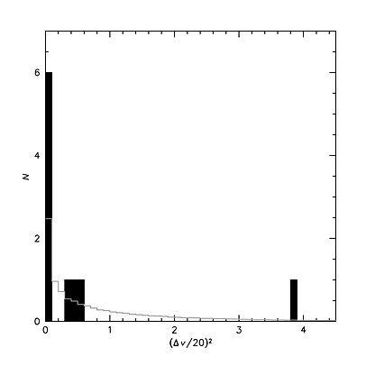
Figure 7. Distribution of the square of the velocity offsets, which is how most estimators of scale "see" the data. The x-axis is normalized for σ=20 km/s. The point at right is GC-98. The grey histogram shows the expected distribution for a Gaussian. For σ=20 km/s, 68% of the data points are expected to lie at <1, and 32% are expected to lie at >1. The observed distribution is non-Gaussian, which means measures such as the rms are biased.
As a result of the extreme distribution in Fig. 7, different estimators for the observed dispersion give wildly different answers: the normalized median absolute deviation gives σ=4.7 km/s and the rms gives σ=14.3 km/s! According to Beers et al. (1990), the least-biased estimator in these situations is the biweight (see section VIb, "Small N (N=10)"). The biweight is identical to the rms for a Gaussian distribution but it does an iterative and objective outlier analysis. It is perhaps the most widely deployed estimator of the scale of a distribution; as an example, anyone who has used robust_sigma in IDL has used the biweight. The biweight estimator identifies GC-98 as an outlier and returns σ=8.4 km/s for the most likely value of the observed (that is, smoothed with the errors) dispersion.
However, what we are after is not the observed dispersion, but the intrinsic dispersion. Or rather, we want to know what range of intrinsic dispersions is consistent with the observed distribution of velocities. In this analysis we want to explain two things: the narrow observed distribution of 9 out of 10 objects, and the presence of the outlier. Note that this is somewhat unusual; often outliers are simply removed (see, for example, Martin et al. (2016) who robustly identify an extreme outlier in their sample of 10 stars). As detailed in the Methods section, we end up with a fairly narrow range of possible intrinsic dispersions:
The upper limit comes from the following simulation: we ask "how likely is it to measure a biweight dispersion <=8.4 in a sample of 10 objects with the observed error distribution if the true dispersion is X?". The lower limit comes from the outlier; here we ask: "if the true dispersion is X, how likely is it to have at least one object in the sample that is at least 39 km/s removed from the mean?". If the underlying (as opposed to observed) distribution is Gaussian, there is only a very limited range of dispersions for which both probabilities are >10%. I should say that I chose this method because it seemed the most obvious thing to do, not because this is on the bleeding edge of statistical analysis. However, as it happens (and as discovered by Yotam), what I did is a version of Approximate Bayesian computation (ABC). I won't pretend I knew this at the time - I've simply always preferred simulations over ML methods for "drawing" problems such as these - but as shown below this enables us to make some detailed comparisons to the ML approach used by Martin et al. I should also note that the lower limit given above only appears in the Methods section of the paper. In the text we only use the upper limit of 10.5 km/s, as that is what constrains the halo mass. However, I recognize that this has led to some confusion that could have been avoided (see Martin et al. 2018).
Martin et al. (2018) take a different approach; they employ a straightforward ML analysis using a likelihood function for a Gaussian distribution with heteroscedastic Gaussian errors. We first note that, given the observed (as opposed to intrinsic) non-Gaussianity, the choice of a Gaussian likelihood function - while perfectly fine in a wide variety of cases - might produce results that are hard to interpret. We will return to this below. However, despite the difference in methodology, Martin et al (2018) find the exact same value for the most likely velocity dispersion as we do. They find
This obviously falls right in the middle of our range. For context, two numbers are of particular relevance: the expected velocity dispersion from the stars alone, which is about 8 km/s (with an uncertainty of perhaps 2 km/s due to systematic uncertainty in the stellar M/L ratio), and the expected dispersion from a normal dark matter halo, which is 30-35 km/s. This is also the average dispersion of Local Group galaxies of the same stellar mass. Therefore, our study and Martin et al. are fully consistent in the central results: 1) the most likely dispersion is nearly equal to that expected from the stars alone; and 2) the data rule out a normal dark matter halo. This is shown explicitly below, where we repeat Fig. 4 from the Nature paper but now using the Martin et al. (2018) velocity dispersion measurement.

Figure 8. Repeat of Fig. 4 from the Nature paper, but now using the Martin et al. (2018) measurement of the velocity dispersion rather than our own. The results are nearly identical, although with a larger error bar.
The uncertainty in the Martin et al. dispersion is larger, leading to a larger range of possible halo masses. This will be discussed below but here we emphasize that, even with the Martin et al. errors, DF2 is quite far removed from the stellar mass - halo mass relation. This is illustrated in Figure 9 below, which shows just how far off the velocities are from the expectation of other Local Group galaxies and from Dragonfly 44: this is not a subtle result. With the Martin et al. dispersion the ratio between halo mass and stellar mass is of order unity and consistent with 0, just as we found.
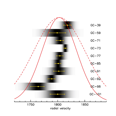
Figure 9. Same as Fig. 5, but now showing the expected velocity dispersion if this galaxy was similar to the average of Local Group galaxies of the same mass (solid red line), or to the UDG Dragonfly 44 (broken red line).
Detailed analysis of the uncertainties in the velocity dispersion
Although there is agreement that the most likely dispersion is close to that expected from the stars alone, our 90% upper limit is lower than the 84% upper limit from Martin et al. Furthermore, Martin et al give a second estimate in their section 2.4.1 that is significantly higher than their default one: 12.0 km/s for the best-fit, biweight-measured, intrinsic dispersion. These differences are small, but they are important: there are several suggested dark matter-less galaxies in the literature (see, for instance, Collins et al. 2013), and if we are claiming that DF2 is a more robust candidate than these previous ones we have to worry about the tails of the distribution. Here we go into a bit more detail to better understand these differences. We don't fully resolve them, but we come a bit closer, hopefully.
We first briefly address the dispersion of 12.0 km/s, as its origin seems clear. This value is of course a bit odd, as the directly measured biweight dispersion is 8.4 km/s, before correcting for the broadening due to measurement errors. The reason for this high value appears to be that the data are resampled in 2.4.1: the measurement is done on realizations of the data that are created by perturbing the measured values according to their error bars. That is mathematically identical to a smoothing by the errors, as can be verified easily. This means that the error bars are applied twice: first in going from the true velocity to the measured velocity, and then in going from the measured velocity to the perturbed velocity. It is the same as smoothing an observed, already PSF-convolved image by the PSF. In the analysis of the perturbed velocities the errors are taken into account only once, leading to an erroneous "intrinsic" dispersion. (It is in fact more akin to the measured dispersion, in the sense that it is a once-smoothed version of the intrinsic distribution, although not quite the same as information is lost in the process of smoothing and fitting). Random realizations of data can be obtained by, for instance, bootstrapping, but not by perturbing the data: that just gives a distribution that is smoothed twice by the errors. I believe that the analysis in 2.4.1 may be in error; but hopefully this will be decided one way or the other in the refereeing process.
We now analyze the differences between the default approach in Martin et al. and the one in the Nature paper - with thanks to Yotam, who really delved into this issue. We concentrate on the upper limit on the dispersion as that is the relevant number for constraining the amount of dark matter. First, we show that the simulation-approach of the Nature paper produces very similar results as the MLE when it is repeated with the rms (rather than the biweight) as the statistic. As a stand-in for the method in the Nature paper we use the ABC (introduced above), as it produces probability distribution functions that can be compared directly to other methods. (We verified that the confidence intervals are very close to those obtained in the Nature paper.)

Figure 10. Comparison of the ABC and MLE methods to determine the intrinsic velocity dispersion. The PDF of the MLE is similar to that obtained by Martin et al. (2018).
The blue curve in Fig. 10 is our PDF of the likelihood; it is similar to that obtained by Martin et al. (2018). For completeness we also ran an MCMC implementation to determine the PDF, as this is also done in Martin et al; however, as the parameter space is limited and well behaved there is no particular advantage to this approach and we find identical results. The orange curve in Fig. 10 is a close match to the blue curve, which shows that ABC produces similar results as the likelihood estimator when the rms is used as the statistic to judge whether simulated distributions are consistent with the observed one. The peak is at approximately 12 km/s, which makes sense as this is the error-corrected value for the rms given in the Nature paper. The other curves in Fig. 10 show the results of ABC when various robust measures of scale are used. These are all consistent, providing 90% upper limits of about 10 km/s (for the biweight) or less (for sigmaG and NMAD). These small differences occur because the biweight calculates the rms of 9 of the 10 objects, whereas the other methods focus on the mid point of the distribution of offsets (which is 3 km/s).
We now ask what happens when GC-98 is removed from the sample. As noted in Martin et al. (2018), this has an effect on the MLE but not dramatically so - without this object they find σ=6.8 km/s, with an upper 1σ error bar extending to 11.4 km/s. We reproduce this result too, as shown by the blue curve below:
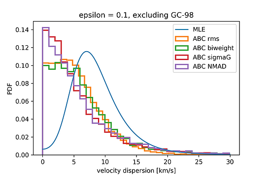
Figure 11. Same as Fig. 10, but now excluding GC-98. The ABC now produces fully consistent results, even when the rms is used as the statistic.
We see that the ABC+rms, which was a good match to the MLE for the full sample, is now fully consistent with all other measures of scale and produces a much more tightly constrained upper limit than the MLE. We note, of course, that intrinsic dispersions less than about 8 km/s are not physical as that is the expectation from the stellar mass alone. This value is within the 1σ confidence limits of all models (both those shown here and those of Martin et al.).
All these ABC implementations (rms, biweight, sigmaG, and NMAD) assume an underlying Gaussian distribution. We can relax that assumption by using a chisq statistic to compare the simulated to the observed distributions. This is done below; again the likelihood method is in blue. This is for all ten objects:
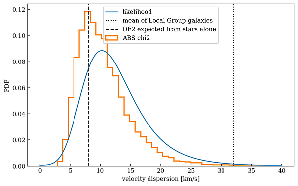
Figure 12. Comparison of the ABC with a chisq criterion fo compare distributions, for all ten objects. The dashed line is the expectation from the stars alone, without dark matter.
Here the dashed and dotted curves indicate the two relevant dispersion expectations: stars only (dashed) and the average of Local Group galaxies of the same stellar mass (dotted). The peak of the orange curve coincides with the expectation for stars alone, even when the full dataset of all ten objects is used. If GC-98 is excluded, the likelihood and ABC+chisq methods produce identical results:

Figure 13. Same as FIg. 12, but now when excluding GC-98.
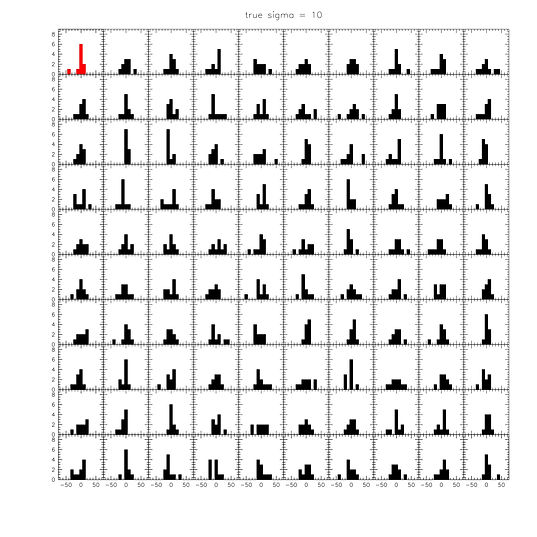
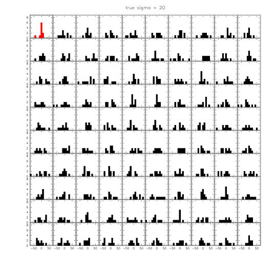
Finally, we provide simple simulation outputs to visually illustrate what is going on. These are 99 simulated observed distributions, drawn for intrinsic dispersions of 0, 10, and 20 km/s. The red distribution is the observed one. For 0 km/s, the peaks are similar to the observed one, but there are very few cases where we see an outlier as large as GC-98. For 10 km/s, we see about 10 distributions with similar peaks as observed - this is where the 90% upper limit comes from in the Nature paper and the ABC method. For 20 km/s, we see plenty of GC-98-like outliers, but we don't have the narrow distribution of the other 9 objects. Anybody can repeat this exercise trivially. First draw 10 velocities from a Gaussian with a particular intrinsic dispersion. Then draw 10 errors from 10 Gaussians, with the σ of each Gaussian set equal to the error for that object. Add the errors to the velocities, and plot the distribution. Then repeat 100 (or 1000) times. These simulations are completely independent of the methodology to measure the dispersion - they simply show what distributions one can expect given an intrinsic dispersion and the observational errors.
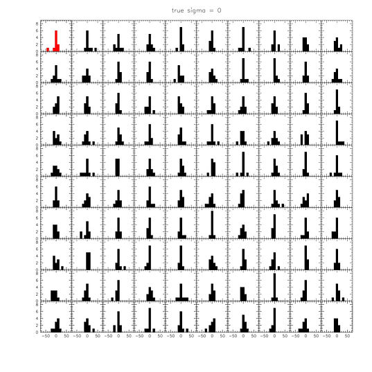
Figure 14. Simulated velocity distributions, for intrinsic dispersions of 0 km/s (top), 10 km/s (middle), and 20 km/s (bottom). The observed distribution is in red.
How reliable is the velocity of GC-98?
Given the importance of GC-98 - see above - it is worthwhile to examine its spectrum in a bit more detail. Below are three objects: GC-73 at the top, which has the highest S/N of the 10, and then the two objects with the lowest S/N, GC-98 (middle) and GC-101 (bottom). GC-101 has a higher formal error than GC-98, but it's clear that the spectrum is much better behaved. GC-98 has a strong negative feature (a factor of two stronger than the expected absorption) at 8592 Angstrom, and a strong positive feature just redward of that (at 8597 Angstrom). The combination of these two features drives the best fit to relative low values. The red CaT line (right panels) also looks suspicious, with a consistent negative residual from 8715-8725 Angstrom. Note that the measured velocity offset is the difference between the location of the red feature and the vertical dashed line - this is a difficult measurement!

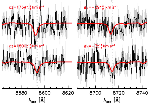
Figure 15. Details of Fig. 2 in the Nature paper. The top spectrum is GC-73, which has the highest S/N ratio of the 10 objects. The other two are the objects with the lowest S/N ratio: GC-98 (middle spectrum) and GC-101 (bottom spectrum). Although the formal errors are larger for GC-101, the GC-98 spectrum has significant systematic residuals in the CaT region.
The bottom line is that the spectrum of GC-98 is the worst of the lot, as it has low S/N and significant systematic residuals that are not seen in the other spectra. This is not a reason to reject it, but this is one possible explanation for its outlier status. Hopefully this will inspire others to remeasure this velocity, and also those of the other objects.
What about MOND?
The original version of the paper had the predicted MOND dispersion in the abstract, but the Nature Editor suggested taking that comparison out and just ending with the finding that dark matter is apparently separable from normal matter on the scale of galaxies. I followed his advice but left the comparison in the main text - perhaps unwisely, given the attention that this aspect has gotten.
The whole MOND / alternative gravity discussion in the paper rests on a misunderstanding on my part. I thought that MOND and Emergent Gravity have no trouble reproducing previously observed objects with large amounts of (apparent) dark matter, in particular Local Group dwarfs and ultra-diffuse galaxies such as Dragonfly 44. As Stacy reminds us, don't bet against MOND when it comes to galaxy dynamics - so I figured (without a careful check) that MOND has no trouble with these previous observations. Starting from that, the huge difference between Dragonfly 44 and the Local Group dwarfs on one hand, and NGC1052-DF2 on the other (see Fig. 4), seemed to rule out MOND, Emergent Gravity, and really any other alternative to dark matter.
The fact that the MOND dispersion for an isolated galaxy with the mass of NGC1052-DF2 is only 20 km/s, not 30+ km/s, should have given me pause, but as even 20 km/s is so much higher than the 10.5 km/s upper limit we derive this did not seem to matter much. However, the MOND prediction may actually be even lower than this, due to the "external field effect" (EFE). Stacy McGaugh wrote about this in the context of DF2, and I won't repeat his arguments here, but the basic idea is that in the MONDian Universe the influence of galaxies extends far beyond their borders and the elliptical galaxy NGC1052 could push DF2 closer to the Newtonian regime. This is actually rather neat, as it provides very different predictions for the behavior of isolated galaxies versus galaxies in dense environments. Unfortunately the actual calculation is difficult, and virtually impossible in dense environments as every galaxy influences every other galaxy. It also requires knowledge of the masses and 3D distances of all neighboring galaxies.
Now, I did actually consider the EFE - I had seen Stacy's nice 2016 paper about the "feeble giant" Crater II, and calculated the EFE dispersion using Eqs. 2 and 4 in that paper. The result, for the values given in the Nature paper, is 25 km/s - higher than the isolated prediction of 20 km/s. It seemed the galaxy is not in the EFE regime and that seemed to be the end of it. After publication of the Nature paper Famaey et al. wrote a paper that performs a more complex calculation, and conclude that the EFE is actually important for this galaxy. The predicted dispersion is lowered from 20 km/s to about 14 km/s (I believe this is for the maximum EFE, that is, for the minimum possible distance to NGC1052). This is still higher than our upper limit of course, but it is closer (see Figs 9 and 10). The Nature paper should have at least mentioned the EFE and the fact that the McGaugh (2016) prescription for the effect says that it is negligible. I'm still not quite sure why this changed so much in the Famaey, McGaugh et al paper, but I will note that Stacy also initially thought the EFE is negligible. In an email, he wrote "indeed, my first thought was that the EFE was unlikely to be important, for the reasons you give."
In any case, the essence of the UDG argument against alternative gravity is scatter: other than is the case for, say, spiral galaxies there appears to be enormous variation in the kinematics of this class of galaxies, and this poses a serious challenge. On the other end of the spectrum from DF2 is Dragonfly 44; this galaxy, as discussed in a 2016 paper, is even larger than DF2, has a similar stellar mass, and a velocity dispersion of 47 +- 7 km/s. It lives in the Coma cluster - I imagine the EFE is important there, also, but even if it isn't, the dispersion is significantly higher than even the isolated MOND prediction (about 22 km/s for Dragonfly 44). The key issue for alternatives to dark matter is the difference between NGC1052-DF2 and Dragonfly 44, as highlighted in Fig. 8. If a theory is able to fit one object, it will have a hard time fitting the other. This is what we should have said more clearly in the paper - my misunderstanding was that I thought MOND could fit Dragonfly 44. (There are always "outs" of course: for Dragonfly 44 those might include measurement errors, non-equilibrium of the galaxy, and perhaps some form of cluster-specific unseen matter).
Globular clusters as mass tracers
Mike Boylan-Kolchin suggested that globular clusters are suspect tracers of the mass, as the kinematics of the five GCs of the Fornax dwarf spheroidal suggest ~zero dark matter. This argument was repeated by Michelle Collins, among others. The reference Mike gives is Cole et al. (2012); this is one of many papers that try to explain the existence of the Fornax globular clusters. The problem with Fornax's globular clusters is not so much the kinematics, but the fact that dynamical friction should cause them to spiral into the center on a relatively short timescale. This can be mitigated, or avoided entirely, by a core in the dark matter profile. (For DF2 the dynamical friction aspect is interesting too, by the way - we are working on that analysis). I do not find a discussion of the kinematics of the globular clusters in Cole et al., although I may have missed it!
So what are the kinematics? Oddly all tables only list velocities for 4 of the 5; the lowest mass one may be too faint for a reliable velocity. The four velocities are -1.2 +- 4.6, 7.1 +- 3.9, 5.9 +- 3.4, and 8.7 +- 3.6. (this is with respect to the systemic velocity of Fornax). These four values are entirely consistent with the stellar dispersion of about 12 km/s: there is a 28% probability of having all 4 observed values be <=8.7 km/s if the intrinsic dispersion is 12 km/s. Using the same methodology as we employed for NGC1052-DF2, we would derive a 90% upper limit on the intrinsic dispersion of 18 km/s, comfortably higher than the stellar dispersion. As an aside, globular clusters have of course been used extensively to measure the kinematics of more massive galaxies - ranging from the Milky Way to giant ellipticals.
There is also a curious debate (on twitter, but also in Martin et al. 2018 and Laporte et al. 2018) about the question whether anything can be said about the dispersion when only 10 tracers are available. The answer is, of course, that it depends on what it is that you want to say. If you have 2 measurements that are 100 km/s apart, the dispersion is likely not smaller than, say, 5 km/s. In fact, the late Mark Aaronson famously discovered the existence of dark matter in dwarf galaxies from the radial velocities of 3 stars in Draco. We also point to Martin et al. (2016), who find a velocity dispersion of 2.9 +- 2.1 km/s (and conclude that the object is dark matter dominated), using only 9 stars.
"No dark matter" versus "dark matter deficient"
It is perhaps worth emphasizing that we do not (and cannot) make the claim that DF2 has no dark matter - merely that the galaxy has a far lower dark matter content than expected from the canonical relations between stellar mass and halo mass. The title was carefully chosen, as "lacking" can mean "having none" but also "having too little of". (In fact, in the editorial process the title was briefly changed to "A galaxy without dark matter" but we made sure that was changed back into "A galaxy lacking dark matter".) In the abstract, it is stated that the ratio between dark and normal matter is "of order unity" (as opposed to "of order 100", as is clear from context), and in the main text we state it is a candidate for a baryonic galaxy. Finally, we show in the Methods section that if the rms is used to estimate the velocity dispersion, or it is assumed that the globular clusters are in an infinitely-thin disk, the galaxy is not devoid of dark matter but still very dark matter deficient. I would argue that it does not matter very much: an analogy that I've used when speaking to reporters is that, if you're $300 short, it does not matter whether you have $1 or $5 or nothing at all on you.
This subtlety has gotten somewhat lost in the retelling of course, and I understand the confusion. In any case, I don't think it's going to be possible to completely exclude the presence of dark matter in any galaxy - the uncertainty in the stellar IMF would preclude that, even with exquisite information. Nevertheless, it would certainly be wonderful if we could place even tighter constraints on the dynamical mass and the amount of dark matter in NGC1052-DF2 - see below.
Can we do better?
There are several ways to improve upon our analysis. The first is to reduce the observational errors, in particular for GC-98 and GC-101. The second is to re-observe GC-93. This is the only reasonably bright GC that does not have a velocity measurement: the CaT is not detected in its spectrum. With an additional 5-10 hrs it should be possible to add this 11th object to the analysis. After that, we run out of globular clusters, but there's also the stellar component. We are planning to (try to!) measure the stellar dispersion of NGC1052-DF2 this coming Fall. It will be difficult, but it is clearly important to have an independent check and, hopefully, an actual measurement rather than an upper limit.